Model-free differentiation and integration of measured motion. Get velocity and acceleration from a noisy displacement record, velocity and displacement from a drifting accelerometer, or fuse both channels. No model of the system is used, only a regularity prior on the signal. MATLAB and Python, MIT license.

Code on GitHubTalk slides (PDF)

The problem

Differentiation and integration are the same ill-posed problem

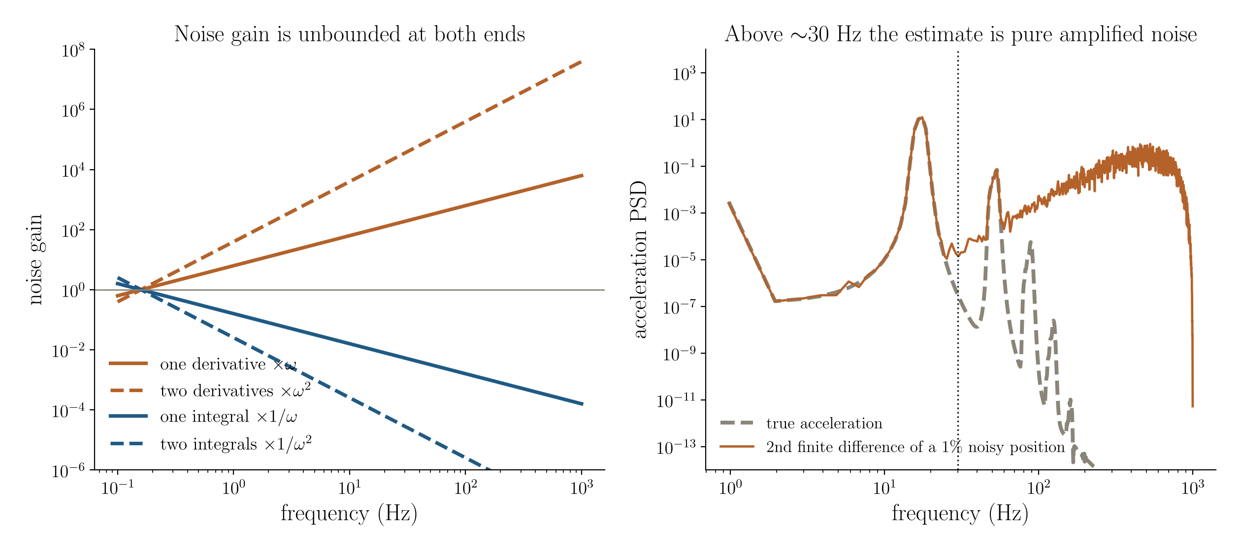
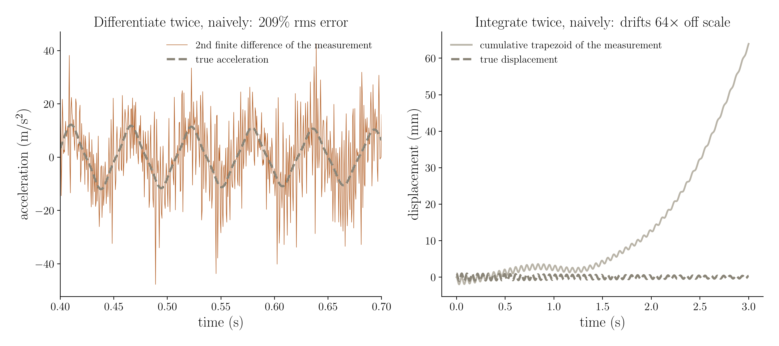
Labs measure displacement (laser vibrometer, DIC, encoder) and need velocity and acceleration, or measure acceleration and need velocity and displacement. Write the measurement as y = Au + e, with A the integration operator. A is compact and its inverse is unbounded, so noise is amplified by ω per derivative and by 1/ω per integration. No algorithm removes this; every usable method adds a regularity prior.

Methods

Pick the prior you actually believe

If you are willing to assume	Use
The signal is bandlimited and periodic	Spectral (FFT) differentiation
It is locally a low-order polynomial	Savitzky–Golay, Lanczos
It lies in a low-rank delay-embedding subspace	SVD / SSA
Its p-th derivative is small in L2	Whittaker–Henderson, Tikhonov, smoothing spline
Its derivative is piecewise constant (L1)	Total variation (Chartrand)
It is an integrated Wiener process	Kalman / RTS smoother (equivalent to a Gaussian process)
Its derivative is bounded by a known constant	Levant sliding-mode differentiator (causal, online)

Benchmark

What the benchmark shows

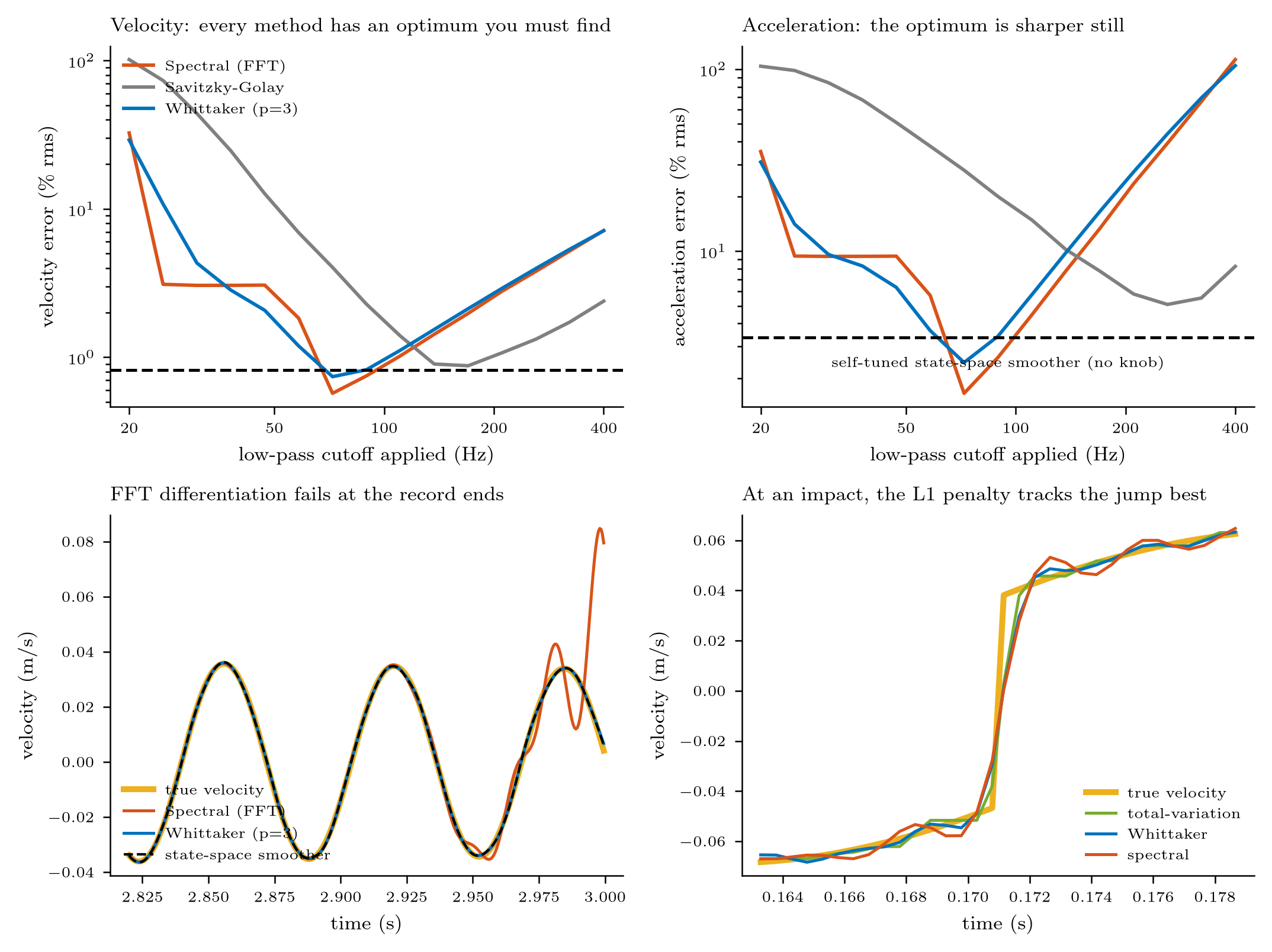
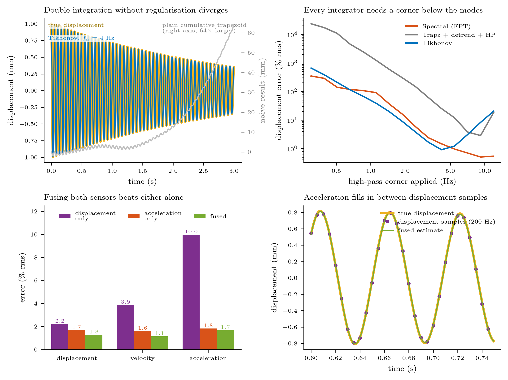
Ground truth is a Duffing free decay (15 Hz, ζ = 0.004, 25% hardening shift at the initial amplitude) sampled at 2 kHz for 3 s. Each method was tuned to its best possible setting; the state-space smoother tunes itself. At 5% noise the self-tuned smoother is within 1.0–1.5 times the error of a perfectly tuned method. The FFT method is the most accurate in the interior of a long record, but its velocity error grows from 0.54% in the interior to 8.4% over the full record because of the ends.

Recommendation

Which method to use

1. Displacement and acceleration channels: fuse them in one state-space smoother. Best accuracy, no cutoff to choose, error bars included, and kinematically consistent outputs.
2. Differentiating a smooth position record, one knob acceptable: Whittaker with p = 3 and a corner frequency set from the physics.
3. Differentiating position with no knob: the self-tuned state-space smoother, nstate = 4 for noisy records, 5 for clean ones.
4. Impacts, stick–slip, backlash: total variation.
5. Acceleration only: Tikhonov integration with the corner below the lowest mode and above the drift. Never a bare cumtrapz.
6. Online or in a control loop: Levant’s differentiator, the only causal one.
7. Long, stationary record whose ends you can discard: the FFT method.

Get started

Using the code

Python (NumPy and SciPy only):

import kinematics as kin

v = kin.diff_whittaker(x, dt, order=1, fc=70)     # velocity from position
d = kin.int_tikhonov(acc, dt, order=2, fc=2.0)    # displacement from acceleration
r = kin.kinsmooth(t, x=x, a=acc, nstate=4, bias=True)   # fuse both
r['x'], r['v'], r['a'], r['std']                  # estimates and posterior std devs

MATLAB (base MATLAB, no toolboxes):

cd matlab; test_kinematics          % verifies the port against the Python reference
v = kin_diff_whittaker(x, dt, 1, 70);
d = kin_int_tikhonov(acc, dt, 2, 2.0);
r = kin_smooth(t, struct('x',x,'a',acc,'nstate',4,'bias',true));

Gaps are NaN, a slower channel is a mostly-NaN column, and non-uniform time is handled directly. The full methods note, tuning rules and cross-validation of the MATLAB port are in the repository README.