Nonlinear Characteristic Value Decomposition: modal identification from a measured or simulated state record, with exact identities, pole correction for numerical derivatives, noise-robust operators, measured forcing, ensembles of records, and amplitude-dependent identification of nonlinear structures. MATLAB and Python, MIT license.

Code on GitHubUser manual (PDF)Live slidesSlides (PDF)Slides (PowerPoint)doi:10.5281/zenodo.23549069

The decomposition

One state record, two identities, both exact

With displacement, velocity and acceleration at $n$ stations, the toolbox writes the state record and its rate as

$$\mathbf{X}_1=[\mathbf{q},\ \dot{\mathbf{q}}]=\mathbf{U}\boldsymbol{\Phi}^{\mathsf{H}},\qquad \mathbf{X}_2=[\dot{\mathbf{q}},\ \ddot{\mathbf{q}}]=\mathbf{U}\boldsymbol{\Lambda}\boldsymbol{\Phi}^{\mathsf{H}}+\mathbf{R}$$

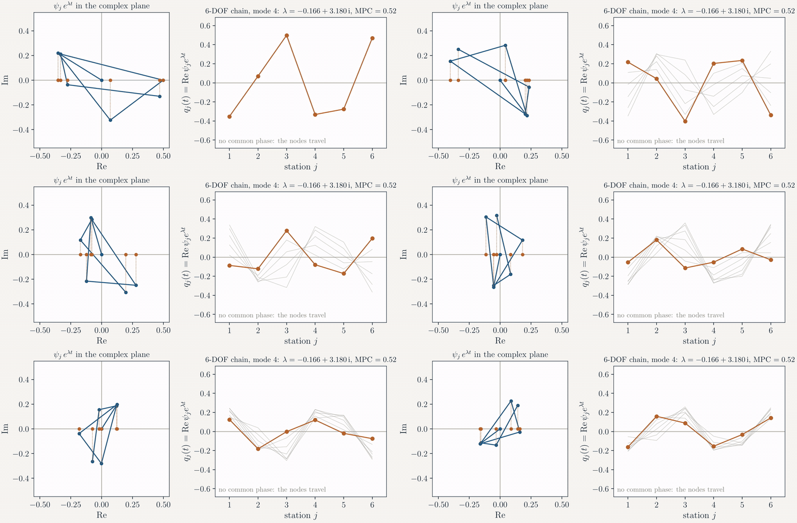
where $\mathbf{U}$ is the temporal basis, $\boldsymbol{\Phi}$ the characteristic shapes, $\boldsymbol{\Lambda}=\operatorname{diag}(\lambda_i)$ the characteristic values (poles) and $\mathbf{R}$ whatever no linear model of the record explains: noise, unmeasured forcing, nonlinearity. The first identity is always exact; the second is exact for a clean linear record, and each pole is paired with its shape by construction.

The readout

Rotating by the eigenvectors of the coupling matrix makes the decomposition exact

The decomposition builds on the characteristic value decomposition (CVD/GCVD) of Li, Stein and Chelidze (2025). It forms the same balanced quotient of second moments and its eigenvectors $\mathbf{V}$, then diagonalises the coupling matrix and rotates:

$$\boldsymbol{\Sigma}_2=\mathbf{V}^{\mathsf{H}}\mathbf{B}\,\mathbf{V}^{-\mathsf{H}}=\mathbf{T}\boldsymbol{\Lambda}\mathbf{T}^{-1},\qquad \mathbf{U}=\boldsymbol{\Xi}\,\mathbf{T},\qquad \boldsymbol{\Phi}=\mathbf{V}\,\mathbf{T}^{-\mathsf{H}}$$

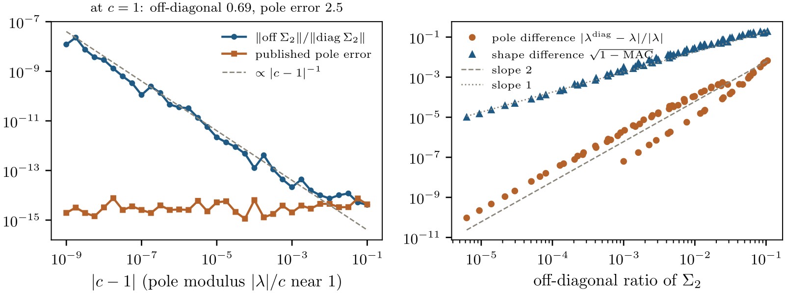
The values are then the eigenvalues of the least-squares state-rate operator $\mathbf{B}=\mathbf{X}_1^{\dagger}\mathbf{X}_2$. Reading them from the diagonal of $\boldsymbol{\Sigma}_2$ instead is exact only when $\mathbf{V}$ already diagonalises it. The balanced quotient applies the Joukowski map $\lambda\mapsto\tfrac12(\lambda+\lambda^{-1})$, which folds the pole plane at the unit circle; averaged ensemble quotients and nonlinear windows also break diagonality. There the diagonal readout errs at second order in the poles and first order in the shapes.

Practical data

Derivatives, sensor noise, forcing and many records

Your data	Use
Displacement, velocity and acceleration	ncvd(d, v, a)
Displacement only	state_from_displacement, then correct_poles
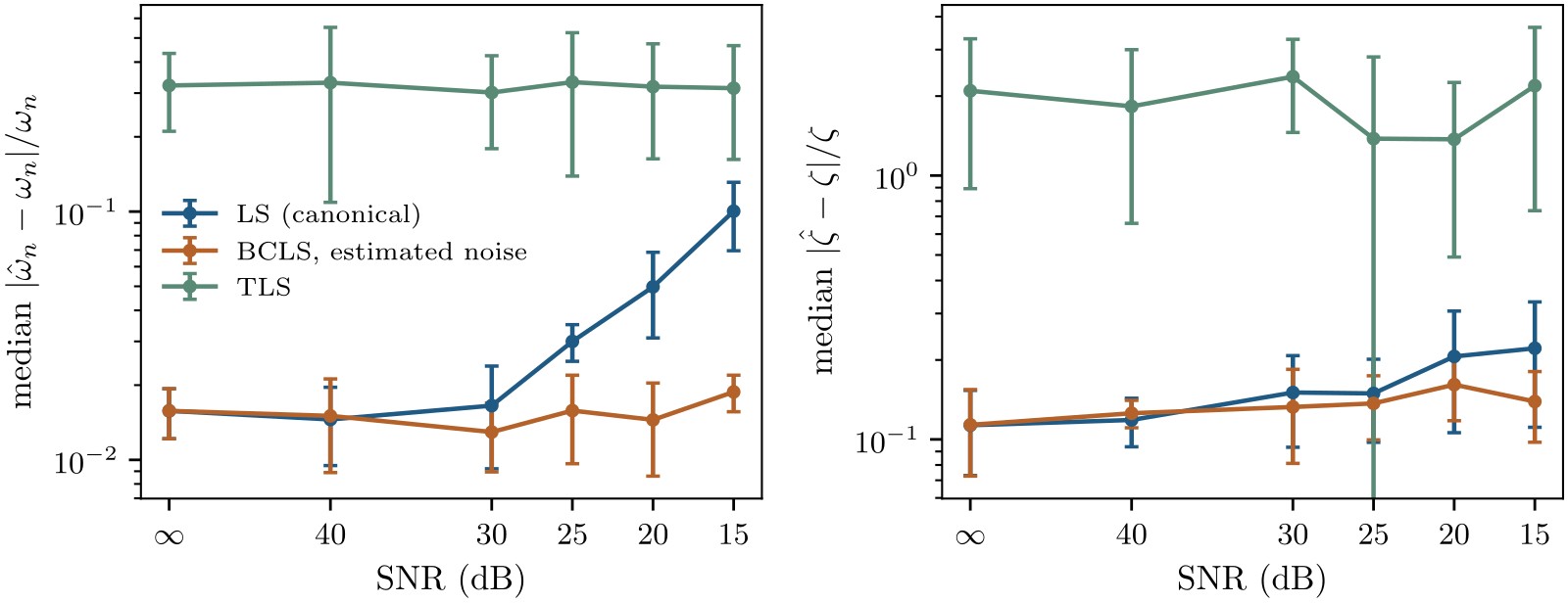
White sensor noise, sampling well above the highest mode	operator='bcls', noise_var='auto'
Measured excitation	forcing=F
Several records at any sampling rates	ncvd_ensemble(records)
Spectrum spanning decades	rank=r
Nonlinear free decay	track(d, v, a, ...)

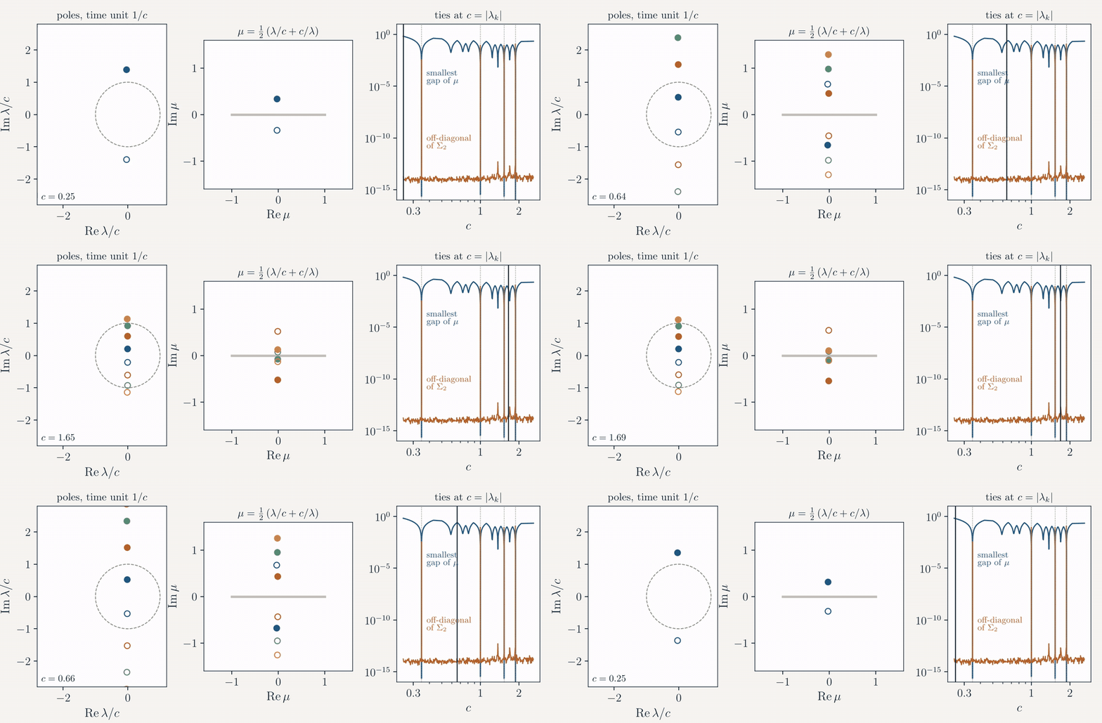
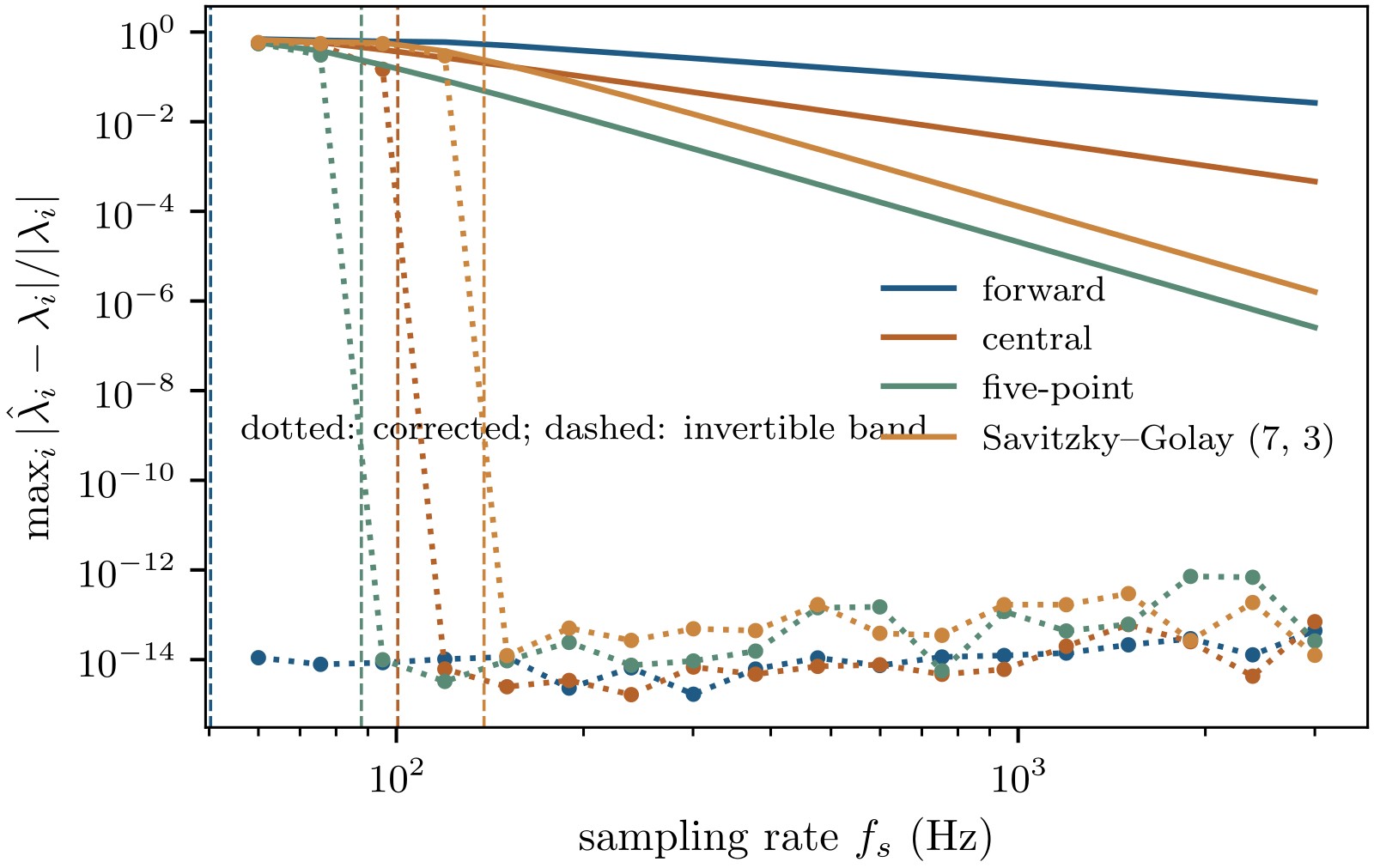
Rates computed from displacement by any FIR stencil return the stencil symbol of the pole, not the pole itself:

$$\tilde\lambda=d\!\left(e^{\lambda\Delta t}\right),\qquad d(\theta)=f_s\sum_j c_j\,\theta^{j},\qquad \lambda=f_s\log\theta$$

Inverting the symbol recovers the pole to machine precision for forward, central, five-point and Savitzky–Golay stencils, inside each stencil’s band.

Nonlinear systems

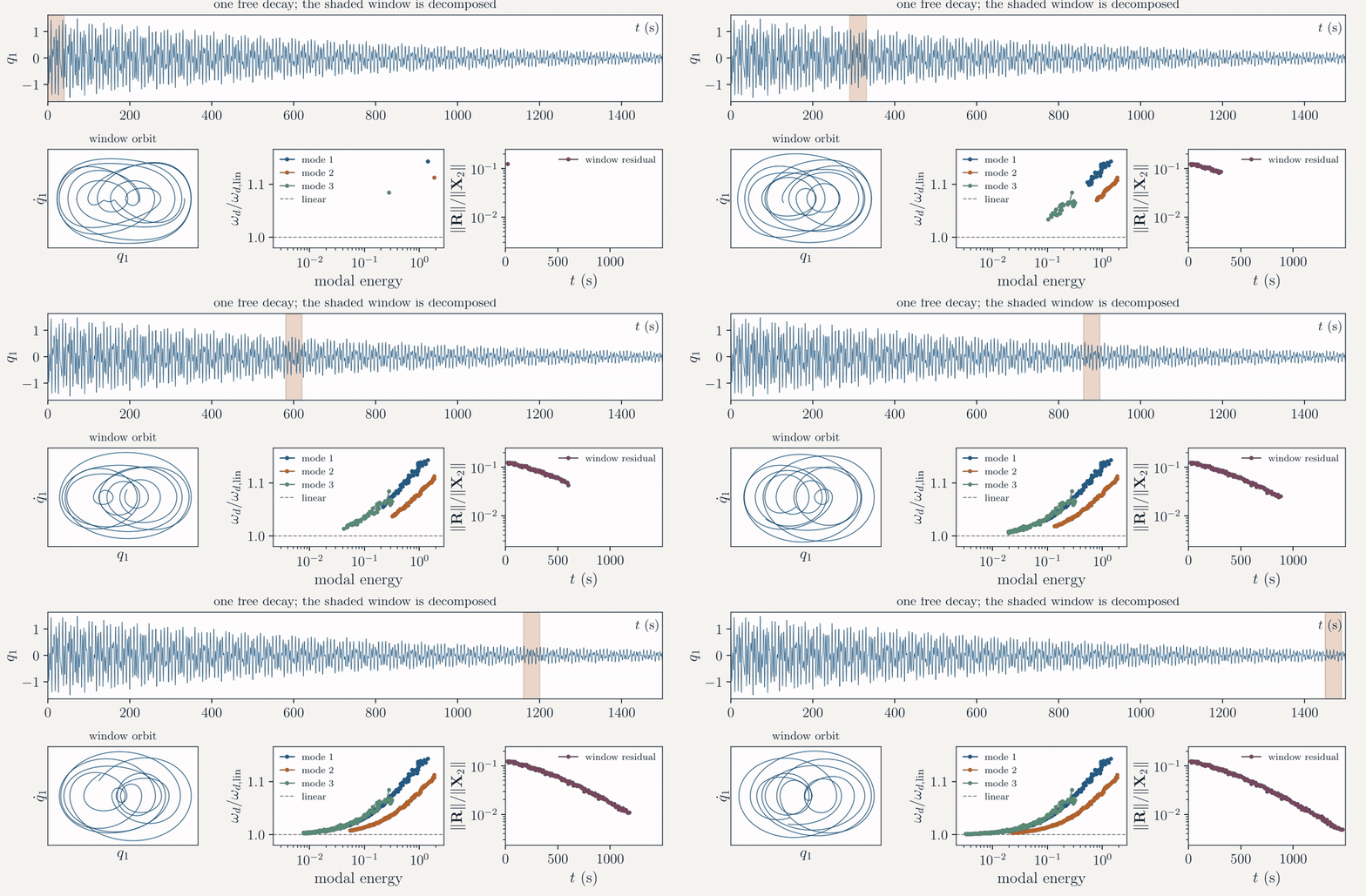
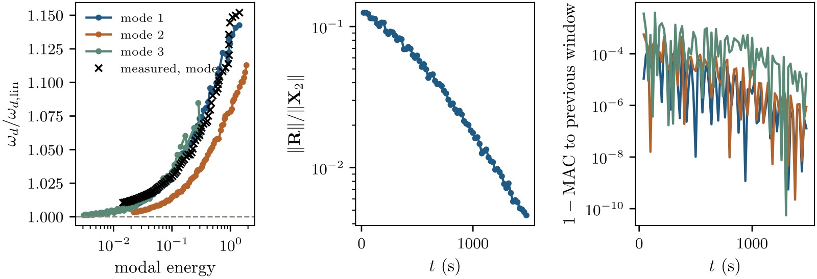
Sliding windows trace frequency-energy dependence from one free decay

Each short window of a decay is decomposed; its values are the best linear description of the local dynamics. Following each resonance through the windows gives the data-driven counterpart of a nonlinear normal mode backbone curve, and the window residual shows how strongly each window engages the nonlinearity.

1. Excite every resonance you track; check the singular values of each window.
2. Span at least one period of the slowest mode per window; a dozen is comfortable.
3. Watch weak modes: a superharmonic of a strong mode can take a weak mode’s pole slot.
4. Validate every pole against the measured response frequency (band_frequency).
5. Trust frequencies and shapes; damping from single nonlinear windows scatters.

Get started

Using the code

Python (NumPy and SciPy):

git clone https://github.com/nld-uri/ncvd-toolbox.git
cd ncvd-toolbox/python && pip install -e .

import ncvd as nc
rec = nc.ncvd(d, v, a)                  # X1 = U Phi^H, X2 = U Lam Phi^H + R
mp  = nc.modal_parameters(rec.lam)      # wn, wd, zeta
tr  = nc.track(d, v, a, fs=fs, length=800, step=400, M=M)   # backbones

MATLAB (base MATLAB, R2022a or later):

addpath('ncvd-toolbox/matlab')
rec = ncvd.decompose(d, v, a);
mp  = ncvd.modalParameters(rec.lam);
tr  = ncvd.track(d, v, a, Fs=fs, Length=800, Step=400, M=M);

Both packages share the same API and are tested against each other. The user manual covers the theory, the options and seven worked examples; the repository README lists the contents.

Citation

How to cite

Please cite both the software, archived on Zenodo as doi:10.5281/zenodo.23549069, and the method paper. ncvd.cite() in Python and ncvd.cite in MATLAB print the entries below.

@software{chelidze2026ncvd,
  author    = {Chelidze, David and Li, Hewenxuan and Stein, Dalton L.},
  title     = {{NCVD} toolbox: Nonlinear Characteristic Value Decomposition for {Python} and {MATLAB}},
  version   = {1.0.0},
  year      = {2026},
  publisher = {Zenodo},
  doi       = {10.5281/zenodo.23549069},
  url       = {https://github.com/nld-uri/ncvd-toolbox}
}

@article{li2025cvd,
  author  = {Li, Hewenxuan and Stein, Dalton L. and Chelidze, David},
  title   = {Characteristic value decomposition: A unifying paradigm for data-driven modal analysis},
  journal = {Mechanical Systems and Signal Processing},
  volume  = {222},
  pages   = {111769},
  year    = {2025},
  doi     = {10.1016/j.ymssp.2024.111769}
}

For amplitude-dependent identification and the reduced-order-model tools, please also cite D. L. Stein, D. Chelidze, Nonlinear Dynamics 113 (2025) 25–45, doi:10.1007/s11071-024-10239-0.