Nonlinear Dynamics Laboratory

Kinematics toolbox

Model-free differentiation and integration of measured motion. Get velocity and acceleration from a noisy displacement record, velocity and displacement from a drifting accelerometer, or fuse both channels. No model of the system is used, only a regularity prior on the signal. MATLAB and Python, MIT license.

Code on GitHub Talk slides (PDF)Live slides doi:10.5281/zenodo.23549236

The problem

Differentiation and integration are the same ill-posed problem

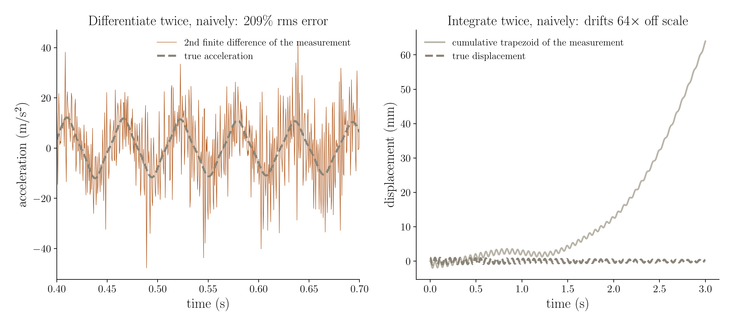
Labs measure displacement (laser vibrometer, DIC, encoder) and need velocity and acceleration, or measure acceleration and need velocity and displacement. Write the measurement as

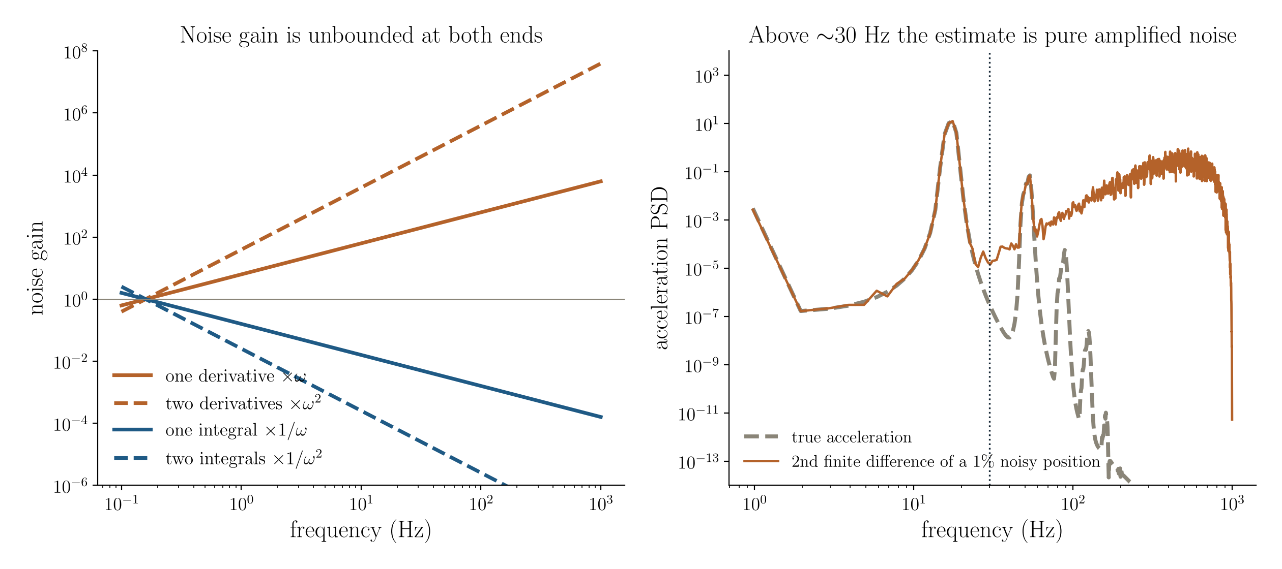
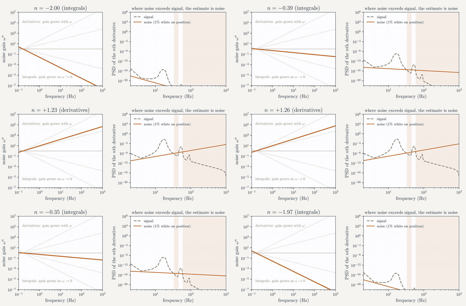
y = A u + e, \qquad (A u)(t) = \int_0^t u(\tau)\,\mathrm{d}\tau

where $u$ is the derivative sought, $A$ is the integration operator and $e$ is the measurement noise. $A$ is compact and $A^{-1}$ is unbounded, so each derivative amplifies noise at frequency $\omega$ by a factor $\omega$ , and each integration by $1/\omega$ . No algorithm removes this; every usable method adds a regularity prior.

Amplification factor of differentiation and integration versus frequency — The amplification is unbounded at both ends. A 1% noise floor on position dominates the acceleration estimate above about 30 Hz.

Animation: noise gain as the derivative order sweeps from two integrals to two derivatives — Animated. Each derivative multiplies the spectrum by ω, each integral divides by it. Left: the noise gain ωⁿ as n sweeps from −2 to +2. Right: signal and 1% position noise after n-fold differentiation; shaded where noise exceeds signal.

Naive finite differences and cumulative trapezoid fail — Ignoring it: a second central difference of 1% noisy position gives 209% rms error; a plain cumulative trapezoid of an accelerometer with 0.5% offset is 64 times off scale after 3 s.

Methods

Pick the prior you actually believe

If you are willing to assume	Use
The signal is bandlimited and periodic	Spectral (FFT) differentiation
It is locally a low-order polynomial	Savitzky–Golay, Lanczos
It lies in a low-rank delay-embedding subspace	SVD / SSA
Its $p$ th derivative is small in $L^2$	Whittaker–Henderson, Tikhonov, smoothing spline
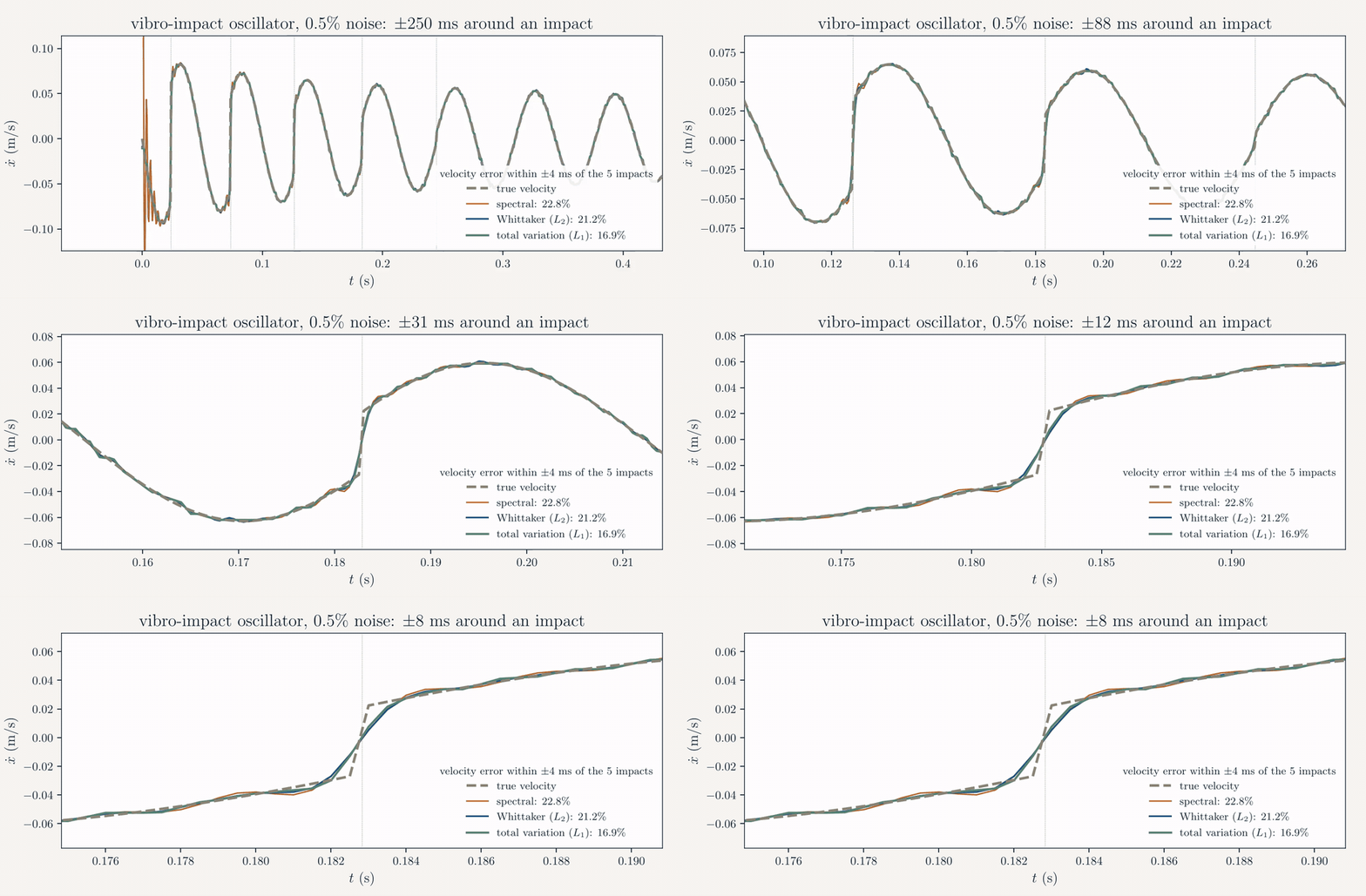
Its derivative is piecewise constant ( $L^1$ )	Total variation (Chartrand)
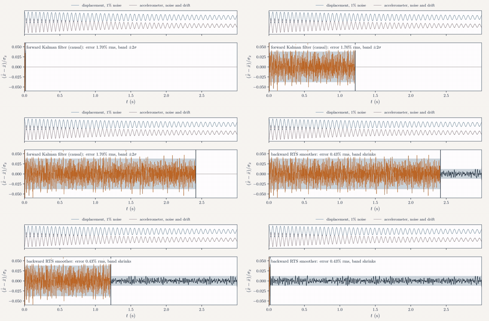
It is an integrated Wiener process	Kalman / RTS smoother (equivalent to a Gaussian process)
Its derivative is bounded by a known constant	Levant sliding-mode differentiator (causal, online)

Benchmark

What the benchmark shows

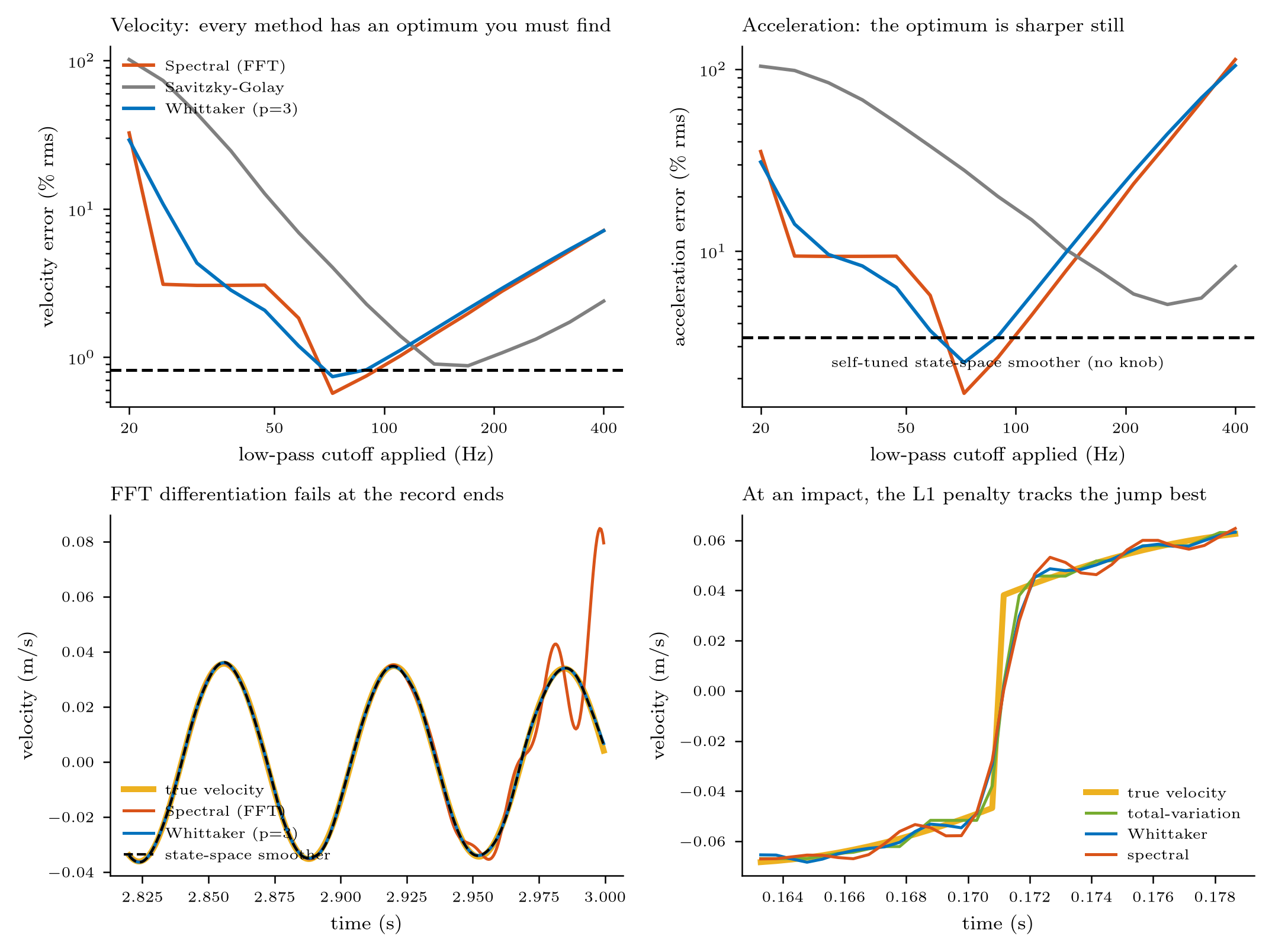
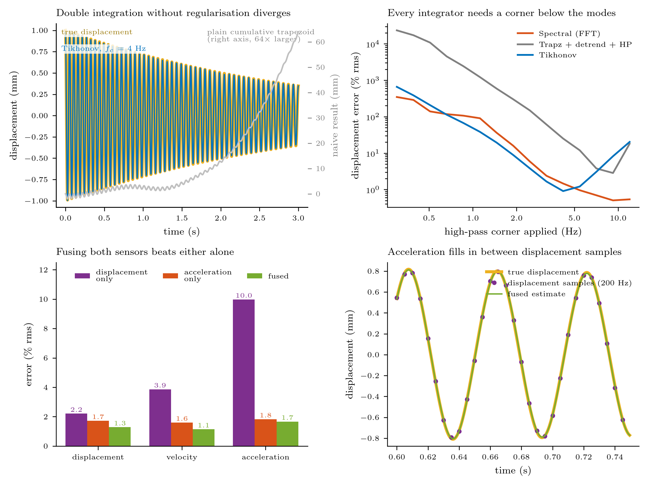
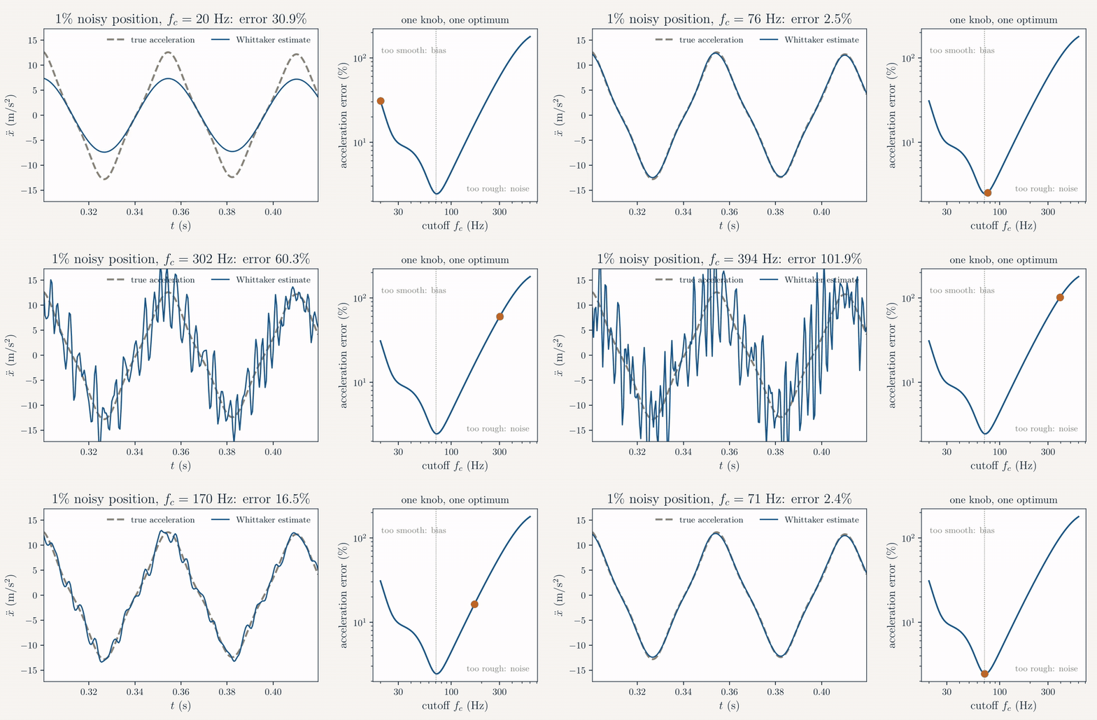
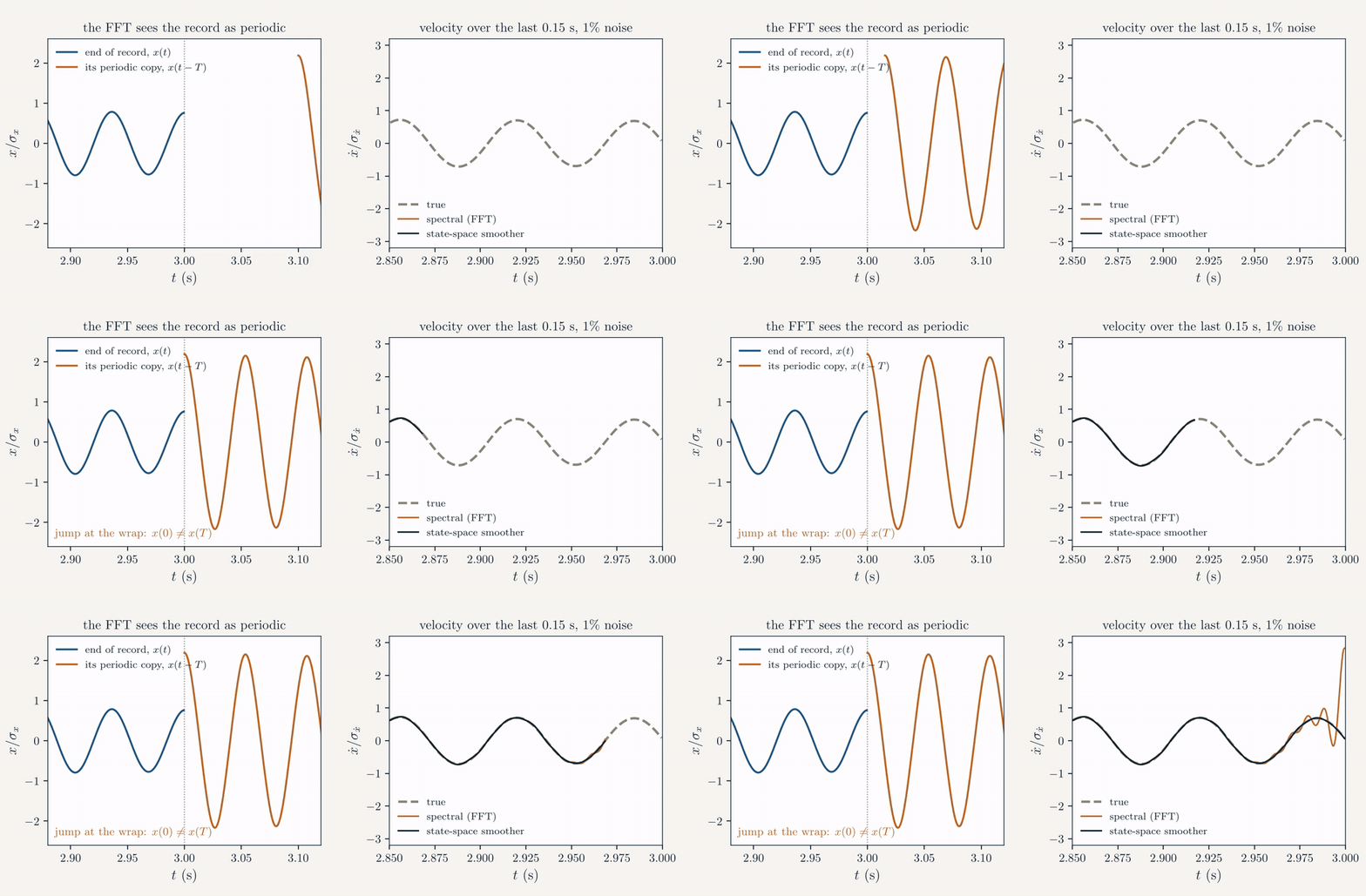
Ground truth is a Duffing free decay (15 Hz, $\zeta = 0.004$ , 25% hardening shift at the initial amplitude) sampled at 2 kHz for 3 s. Each method was tuned to its best possible setting; the state-space smoother tunes itself. At 5% noise the self-tuned smoother is within 1.0–1.5 times the error of a perfectly tuned method. The FFT method is the most accurate in the interior of a long record, but its velocity error grows from 0.54% in the interior to 8.4% over the full record because of the ends.

Velocity and acceleration error of each differentiation method — Differentiation error of each method against noise level.

Integration of acceleration and fusion of displacement and acceleration — Integrating a drifting accelerometer, and fusing it with a displacement channel in one state-space smoother.

Animation: Whittaker acceleration as the cutoff sweeps, with the error curve — The one knob. Whittaker acceleration from 1% noisy position as the cutoff sweeps from 20 to 600 Hz. Too low a cutoff biases the estimate; too high lets noise in.

Animation: the FFT periodic extension and the end-of-record error — Record ends. The FFT treats the record as one period, so the end of a decay meets its own start with a jump. Spectral velocity error reaches 2.7σ at the last sample; the state-space smoother stays below 0.02σ.

Animation: zoom onto an impact of the vibro-impact oscillator — Impacts. Velocity error within ±4 ms of the five impacts, 0.5% noise: spectral 22.8%, Whittaker 21.2%, total variation 16.9%.

Animation: forward Kalman filter then backward RTS smoother fusing two sensors — Fusion. One state-space model fuses 1% noisy displacement with a drifting accelerometer. Forward Kalman pass: 1.70% velocity error. Backward RTS pass: 0.43%. Grey: ±2σ posterior band.

Recommendation

Which method to use

Displacement and acceleration channels: fuse them in one state-space smoother. Best accuracy, no cutoff to choose, error bars included, and kinematically consistent outputs.
Differentiating a smooth position record, one knob acceptable: Whittaker with $p = 3$ and a corner frequency set from the physics.
Differentiating position with no knob: the self-tuned state-space smoother, nstate=4 for noisy records, nstate=5 for clean ones.
Impacts, stick–slip, backlash: total variation.
Acceleration only: Tikhonov integration with the corner below the lowest mode and above the drift. Never a bare cumtrapz.
Online or in a control loop: Levant’s differentiator, the only causal one.
Long, stationary record whose ends you can discard: the FFT method.

Get started

Using the code

Python (NumPy and SciPy only):

import kinematics as kin

v = kin.diff_whittaker(x, dt, order=1, fc=70)     # velocity from position
d = kin.int_tikhonov(acc, dt, order=2, fc=2.0)    # displacement from acceleration
r = kin.kinsmooth(t, x=x, a=acc, nstate=4, bias=True)   # fuse both
r['x'], r['v'], r['a'], r['std']                  # estimates and posterior std devs

MATLAB (base MATLAB, no toolboxes):

cd matlab; test_kinematics          % verifies the port against the Python reference
v = kin_diff_whittaker(x, dt, 1, 70);
d = kin_int_tikhonov(acc, dt, 2, 2.0);
r = kin_smooth(t, struct('x',x,'a',acc,'nstate',4,'bias',true));

Gaps are NaN, a slower channel is a mostly-NaN column, and non-uniform time is handled directly. The full methods note, tuning rules and cross-validation of the MATLAB port are in the repository README.

Citation

How to cite

Please cite the software, archived on Zenodo as doi:10.5281/zenodo.23549236. kinematics.cite() in Python and kin_cite in MATLAB print the entry below.

@software{chelidze2026kinematics,
  author    = {Chelidze, David},
  title     = {Kinematics toolbox: Model-free differentiation and integration of measured motion},
  version   = {1.0.0},
  year      = {2026},
  publisher = {Zenodo},
  doi       = {10.5281/zenodo.23549236},
  url       = {https://github.com/nld-uri/kinematics-toolbox}
}