“Mapping Circulation in the Kuroshio Extension with an array of Current and Pressure recording Inverted Echo Sounders”, recently published in the Journal of Atmospheric and Oceanic Technology, describes a comprehensive methodology to produce mesoscale-resolving 4-dimensional circulation fields of temperature, specific volume anomaly, and velocity from an array of CPIES (Donohue et al. 2010, doi:10.1175/2009JTECHO686.1). This paper consolidates and documents the many advances that have taken place over the past 30 years to interpret IES measurements. Although many of the details in Donohue et al. (2009) are specific to the KESS array, the techniques described are pertinent for analyzing inverted echo sounder, pressure, and current measurements in other regions.
Frequently Asked Questions:
What do IES, PIES and CPIES measure?
- An IES measures vertical acoustic travel time (VATT), also called tau (τ), round trip from the sea floor to the sea surface.
- A PIES adds bottom pressure measurements to an IES.
- A CPIES adds current measurements (50 m above the bottom) to a PIES.
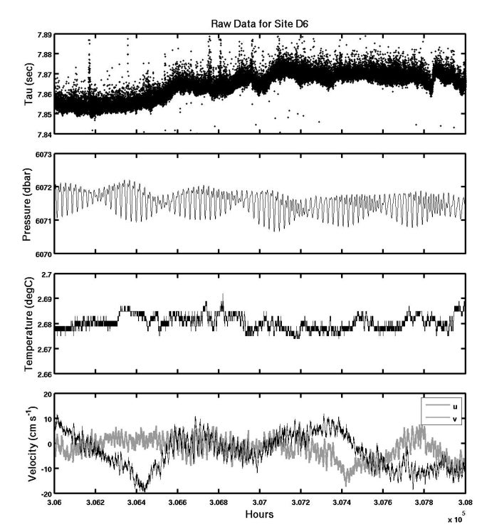
What do raw data look like?
- Example plot shows travel time concentrated in a narrow range of approximately 0.01 seconds, raw pressure dominated by the tidal signal, small temperature variations and small magnitude bottom currents.
How are hourly τ measurements obtained from raw τ data?
- IESs are configured to emit twenty-four 12-kHz pings per hour, in programmable bursts of 4, 8, 12 or 24 pings. A representative travel time for each hour is selected using a quartile method (Example plot: τ burst (blue), hourly τ (red)).
How is τ at one pressure related to τ at another pressure?
- τ at any deep pressure is linearly related to τ at any other deep pressure.
How are τ and thermocline depth related?
- Because the speed of sound is approximately a linear function of temperature, an upward displacement of the main thermocline leads to proportionally less warm water and a lower average speed of sound. This increases τ (Powerpoint Animation: Click on sound source in either water column to begin). Watts and Rossby (1977) describe the first scientific use of IESs to acoustically monitor depth variations of the main thermocline during MODE.
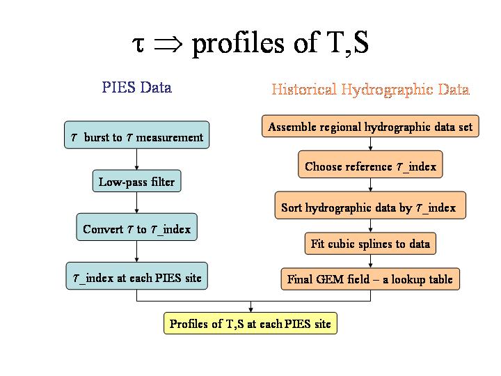
How are τ and temperature, salinity and density related?
- A robust empirical relationship exists between τ and vertical profiles of temperature, salinity and density. These relationships are obtained using historical hydrographic measurements from the oceanic region of interest using the “Gravest Empirical Mode” or GEM method (Meinen and Watts, 2000; Watts et al., 2001b).
How is a GEM representation constructed?
- The flowchart identifies the following steps:
What information can be obtained from multiple IESs?
- Measurements from two IESs can be used, through geostrophy, to determine the vertical profile of the component of horizontal velocity normal to the line between the two IESs. An L-shaped group of three IESs determines estimates of both velocity components. A 2-D array of appropriately spaced IESs can map out the 3-D structure of the horizontal velocity field. Additionally, deep pressure and current measurements can provide referencing to make the velocity profiles absolute.
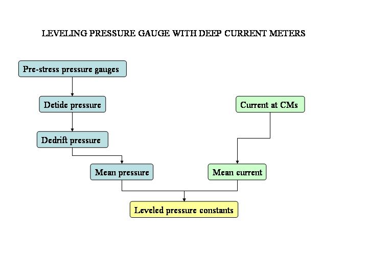
How are PIES/CPIES pressure data processed?
- Pressure data are detided, dedrifted, lowpass filtered and leveled (flowchart).
What is detiding?
- Tidal response analysis (Munk and Cartwright, 1966) determines the tidal constituents for each instrument. Tides are then removed from the pressure records.
What is pressure drift?
- “Drift” refers to a temporal change in pressure calibration.
What is dedrifting?
- Dedrifting removes any drift in the pressure measurentments.
What is leveling?
- Leveling is the technique of referring all measurements onto a geopotential surface. Once leveled, pressure gradients can be used to calculate absolute geostrophic currents.
What are methods for dedrifting?
- Watts and Kontoyiannis (1990) dedrifted bottom pressure by the subtraction of a linear plus exponential curve fitted to each time series. However, their method does not distinguish between instrumental pressure drift and real ocean signals. When deep current measurements are available the new technique described in Donohue et al. (2009) can be used. With this method, ocean signals determined with the measured currents are removed from the measured pressures, and curves are fitted only to the remaining instrumental drift. An advantage of this method is that it simultaneously dedrifts and levels pressure measurements. Figure 5 from Donohue et al. 2009 illustrates this new procedure.
How are maps of daily pressure and current fields generated?
- Maps of the daily pressure and current fields are obtained by combining leveled pressure measurements and current measurements in a multivariate, nondivergent optimal interpolation (flowchart, Watts et al., 2001a).
References
- Donohue, K. A., D. R. Watts, K. L. Tracey, A. D. Greene, and M. Kennelly, 2010, Mapping circulation in the Kuroshio Extension with an array of Current and Pressure recording Inverted Echo Sounders. J. Atmos. Oceanic Technol., 27, 507-527. (doi:10.1175/2009JTECHO686.1)
- Meinen, C.S., and D.R. Watts, 2000, Vertical structure and transport on a transect across the North Atlantic Current near 42 N: Time series and mean, J. Geophys. Res., 105, 21,869-21,892. (doi:10.1029/2000JC900097)
- Munk, W.H. and D.E. Cartwright, 1966, Tidal spectroscopy and prediction, Phil. Trans. Roy. Soc. London, 259, 533-581. (doi:10.1098/rsta.1966.0024)
- Watts, D. R. and H. T. Rossby, 1977, Measuring dynamic heights with inverted echo sounders: Results from MODE, J. Phys. Oceanogr., 7, 345-358. (doi:10.1175/1520-0485(1977)007%3C0345:MDHWIE%3E2.0.CO;2)
- Watts, D.R. and H. Kontoyiannis, 1990, Deep-ocean bottom pressure measurements: Drift removal and performance. J. Atmos. Ocean. Technol., 7, 296-306. (doi:10.1175/1520-0426(1990)007%3C0296:DOBPMD%3E2.0.CO;2)
- Watts, D.R., X. Qian, and K. L. Tracey, 2001a, Mapping abyssal current and pressure fields under the meandering Gulf Stream. J. Atmos. Oceanic Technol., 18, 1052-1067. (doi:10.1175/1520-0426(2001)018%3C1052:MACAPF%3E2.0.CO;2)
- Watts, D.R., C. Sun, and S. Rintoul, 2001b, A two-dimensional gravest empirical mode determined from hydrographic observations in the Subantarctic Front. J. Phys. Oceanogr., 31, 2186-2209. (doi:10.1175/1520-0485(2001)031%3C2186:ATDGEM%3E2.0.CO;2)